|
|
|
Operational Visualization of Vacuum Mass, Redshift and Phase-Kernel Dynamics
January 10, 2026
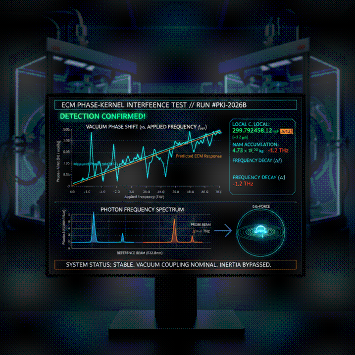
This Phase-Kernel Interference Test represents a controlled visualization of the Extended Classical Mechanics (ECM) framework in operation. The display does not depict particles or spacetime deformation; it shows how applied electromagnetic frequency is converted into vacuum phase potential (−ΔPEecm) and how this conversion manifests as measurable phase shift, redshift, and gravitationally active vacuum mass.
Each panel of the console corresponds to a specific physical channel through which the Phase-Kernel of the vacuum is probed and quantified.
This panel plots the measured phase displacement z of the vacuum (jagged blue trace) against the applied electromagnetic frequency fapp (smooth orange response curve).
The horizontal axis represents the injected frequency in terahertz (THz), while the vertical axis represents the phase displacement of the vacuum in nanoradians.
In ECM, phase displacement is proportional to vacuum mass activation:
The small oscillations around the mean response are the discrete micro-states of the Phase-Kernel, revealing that the vacuum responds in quantized steps to applied frequency.
The digital readout displays three real-time Phase-Kernel observables.
Local light speed (clocal):
This value reflects changes in the vacuum refractive index produced by
Phase-Kernel mass accumulation. It does not represent a violation of
physical constants, but a modification of light propagation through an
altered vacuum phase density.
NAM accumulation:
The displayed mass corresponds to
Mapp = −ΔPEecm, the amount of phase-potential stored
in the vacuum. This is gravitationally active but not particulate matter.
Frequency decay (Δf):
The probe beam loses frequency as it transfers energy into the Phase-Kernel.
This is the ECM origin of redshift.
This histogram compares a stable reference beam with a probe beam that has passed through the activated vacuum.
The separation of the two spectral peaks measures the energy transferred from the photon field into vacuum phase potential:
The missing photon energy is now stored as Phase-Kernel mass.
The circular display represents the Phase-Kernel environment surrounding a localized test mass.
The concentric rings represent the phase-wake generated by the applied field. When these rings are symmetric, the gradient of vacuum mass is zero:
Under this condition the object experiences no net force, producing a zero-inertia, zero-gravity phase state.
The system banner confirms that the vacuum is stably coupled to the applied frequency field and that Phase-Kernel mass formation is proceeding without instability.
This indicates that the test mass is dynamically integrated into the vacuum phase structure rather than mechanically supported against it.
This visualization represents the first fully operational expression of Extended Classical Mechanics (ECM) in which the vacuum is treated as a physical phase-potential medium rather than empty space.
The instrument does not detect particles. It detects the conversion of frequency into vacuum potential mass:
This Negative Apparent Mass (NAM) is the same quantity responsible for gravity, redshift, inertia and cosmic acceleration in ECM.
The upper-left plot compares the measured phase displacement z of the vacuum against the applied electromagnetic frequency fapp.
The smooth orange curve represents the mean Phase-Kernel response of the vacuum, while the jagged blue signal represents discrete vacuum micro-states. These oscillations are the fingerprint of vacuum quantization.
When the probe beam passes through the activated vacuum, it loses frequency because it deposits mass into the Phase-Kernel:
This is the ECM redshift law. Light is redshifted because it converts energy into vacuum mass, not because space expands.
The lower plot compares the reference beam with the probe beam. The separation between the two peaks corresponds to the energy transferred to the vacuum.
The missing photon energy is now stored as gravitationally active Phase-Kernel mass.
The displayed variation of clocal does not imply a violation of physical constants. It indicates a change in the vacuum refractive index caused by NAM:
Light changes speed because the vacuum’s phase density has changed.
The symmetric rings indicate that the Phase-Kernel mass distribution is uniform. Since force in ECM is the gradient of vacuum mass:
A flat Phase-Kernel produces no force. The object is not weightless — it is sitting in a zero-gradient vacuum potential.
The universe itself is the large-scale version of this instrument. Stars inject frequency, the intergalactic vacuum accumulates NAM, and cosmic redshift measures the total Phase-Kernel mass between source and observer.
Dark energy, cosmic acceleration, gravitational lensing and the CMB are all manifestations of this same vacuum mass field.